Engineering Explainability with ML Ops
Adapted from my technical papers: Engineering Explainability into Enterprise AI and Engineering ML Ops into Enterprise AI, both first published in 2021.


Introduction: Risk/Trust
Some of the biggest hesitations in the adoption of AI in the enterprise are due to ethical concerns; businesses hesitate due to the risk of the AI “getting it wrong” and humans hesitate to fully trust in the AI.
Enterprises are unwilling to take responsibility and be held accountable for the consequences of an AI decision that is insufficiently explainable and perhaps counterintuitive. If a decision is counterintuitive and unexplained how do we trust the AI “black box”? Or are we forced to revert back to human decisions? Because even if these decisions are made slower than competitors, at least they’ll be trustworthy. So how is it that competitors are able to move faster with AI-driven decisions?
The root of the answer to all these questions is explainability. Explainability gives businesses the confidence to be accountable for the decisions made. Explainability gives their customers confidence that the decisions have been made in their best interests. Explainability enables the business to take good risks to improve their products, whilst retaining the trust of their customers. So explainability should be a product feature, built into every AI product.
AI systems are realised in the business through software engineering. This paper recommends software engineering methods to create explainability when building AI systems and when subsequently operating them in a real production setting. It starts with a quick look at how complex AI models have an inherent lack of explainability, then at how technology operations should implement explainability in its workflow, and finishes with the various degrees of maturity in AI operations.
Explaining machine learning models: Simple rules, complex systems
The most simple neural network (NN) is very simple indeed; there are only a few parameters that describe it completely, and these parameters can be checked to assure that it has been constructed correctly. But the most simple NN doesn’t do much and isn’t very interesting. It’s when neurones are connected together, with cross-connections, feedback/feed-forward and maybe even memory cells, very interesting neural networks emerge.
These NN can learn for themselves how to interpret information and form decisions, with training. But the fact that they must be trained, not computed, means they produce a complex rule framework which cannot be analysed by examining its components (lacks intrinsic explainability). This black box framework is only empirically accessible, through test and measure (post-hoc explainability).

Image by author.
In developing engineering techniques it is important to examine how the ML model interprets its data separately from explaining how it makes its decisions. Interpretability (metrics for how “easy” it is to derive predictions from data) and explainability (methods for how to relate predictions to data) are closely linked but different. Interpretability is a property of a dataset and should be calculable from the dataset objects. Explainability is a property of a model and should be measurable from the model + dataset objects.
Businesses have some key questions they want to see addressed through model explanations:
How sensitive are the decisions to changes in inputs?
Which inputs is the model most sensitive to?
How transferable is the explanation of the model?
What are the edge cases that the model may be expected to fail?
What can be done to mitigate the impact of such failures?
How did bias creep into the data in the first place?
Explaining datasets and features: Sampled data, biased data
Part of the work of the data scientist is to identify, quantify and mitigate bias. Chief of the sources of bias is in sampling.
At the scale of enterprise data problems, of ML models applied to arbitrarily large datasets, training models on the full dataset is undesirable due to the computational cost, so models are trained from samples. But whenever a sample is used, unless it is truly representative, it will be biased. So the key question becomes: how can we use the available, presumptively biased dataset to generalise predictions to new unseen datasets?
An engineering approach answers this question in two parts: first quantify the bias so that users can make an informed judgement as to how to use the data (acceptable bias); then predict the effect of bias so that users can make informed judgements as to how to use the predictions.
One can tell whether a dataset is biased by comparison; if two datasets, sampled from the same source data, have different distribution metrics then we can see that one is biased from the other. The flip side is that it is impossible to identify bias by computing the raw numbers of a single dataset without making a comparison. Calculating comparative marginal distribution of features and comparative conditional probability distribution of two features quantifies such domain divergence.
Impact of dataset bias on model predictions
Once we expect datasets to be biased due to sampling effects, understanding the impact of bias becomes the next step. The enterprise ML model should give guidance to its users as to whether the differences are acceptable, whether it’s safe to use the training data on unseen live data.
The natural next question is how the features are used in the trained model. The Partial Dependence Plot (PDP) shows how varying an “input” feature impacts the model response. It computes to a single value (commonly the average) all the samples corresponding to the x-axis value being plotted. A PDP can therefore help explain how each feature of interest (as per prior tagging, as described earlier) impacts the model’s prediction.
Comparing PDP plots of features answers explainability questions about single journeys (e.g. predictions about one person) through the model:
Which feature influences the model the most?
Is the amount of influence consistent over the distribution of feature values?
Do features have undue influence?
At what threshold value (of the feature) does the model prediction change? (Informative for categorical ML models.)
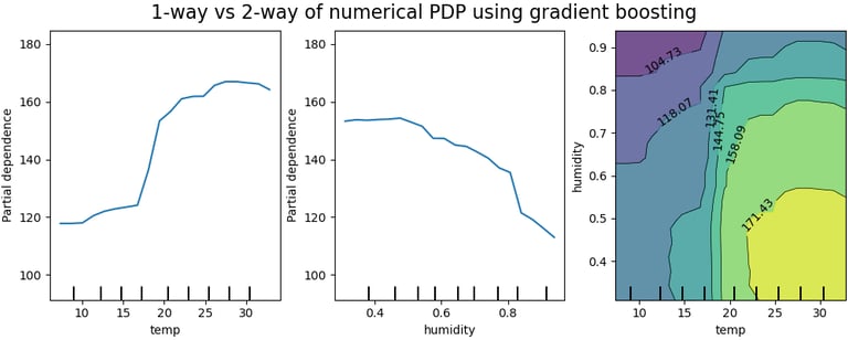
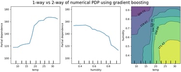
Image © 2007 - 2023, scikit-learn developers (BSD License).
Individual Conditional Expectation (ICE) plots take this a step further. An ICE plots along the y-axis the model prediction for every sample of the dataset corresponding to the x-axis value being plotted. In this way, the distribution of contribution of the feature can be visualised, not just the average. Comparing ICE plots answers the further explainability questions across all journeys (e.g. full population) through the model:
Which features contribute high variance (equating to high uncertainty) in the prediction?
Which features have significant outliers (which merit special treatment) in the prediction?
Are the outcomes equitable for the full population being served?
Image © 2007 - 2023, scikit-learn developers (BSD License).
All of these questions together answer whether bias makes a difference to the computed prediction, by explaining how the feature contributes to the prediction. But both these types of plots are computationally expensive and don’t work well on sparse datasets (as is often the case with fused datasets).
In a real-world solution, it’s no good to deliver bias measurements separately and later than the decisions themselves. This is where an ML engineering approach should implement approximation techniques that yield good results but more efficiently. By reducing the computation load, explainability is presented in near-real-time, so as to fit in with the user’s workflow.
Explainability and privacy
At this stage it’s appropriate to inject some caution; we can’t trade explainability for privacy. For example, whilst we must be able to say how a particular feature influences a prediction, we mustn’t be able to say how a particular data point (person) influences the prediction. To protect privacy, we must implement differential privacy:
Imagine you have two otherwise identical databases, one with your information in it, and one without it. Differential Privacy ensures that the probability that a statistical query will produce a given result is (nearly) the same whether it’s conducted on the first or second database.
This is a rigorous mathematical treatment of privacy and helps us to develop engineering approaches. One such approach is to inject noise into the decision. By making the decision less precise, it is less likely to be able to trace backwards to the input. Engineering questions to investigate:
How much noise should we add?
Does this noise addition vary with processing of dataset (e.g. relationship with features used)?
How do we make this calculation without having information about the dataset (and so introduce bias)?
Which metric best calculates the trade-off between noise and accuracy, i.e. between explainability and privacy?
Fitting explainability into an ML Ops workflow
In 2008, Google introduced its Flu Trends model that predicted the percentage US population with influenza, in time and geography. For a number of years, it outperformed the US CDC predictions, as it fused a wider range of datasets notable search terms. The exception was in 2012, when the model fell very short, demonstrating that even the most well-funded ML model can suffer if not maintained in life. Explainability is not a one-time action, assessed by audit at the time of training the ML model.
ML Ops isn’t just the new DevOps
The IT industry has benefitted tremendously from the previously disparate disciplines of software development and operations becoming closely coupled. It’s now no longer revolutionary, but obvious that software should be written to be deployable and operable in as efficient way as possible. So it’s no surprise that the ~Ops suffix is applied to machine learning software as well.
The bad news is that simply applying the exactly the same approach from DevOps to ML model development and deployment doesn’t result in ML Ops. There are entirely new considerations in ML model development that need to be considered. Further bad news is that DevOps and ML Ops alone do not make a successful deployment. Our maturing understanding defines a suite of xOps capabilities to master:
DevOps - closely coupling software development with its deployment and ongoing operations
DevSecOps - placing security at the heart of DevOps
DataOps - the development and operations of how data is (continuously) sampled, cleaned, labelled, joined, presented and archived
ML Ops - closely coupling model development and deployment with that of software applications and data pipelines; the capability to deploy and observe the right model + right data + right application, at the right time.
Challenges to be addressed by ML Ops
Financial services is an industry where the use of ML models can have a huge beneficial impact, but with an equally large negative impact if things go wrong. The Bank of England released a survey on the state of machine learning in UK which described the challenges in the deployment of ML models, and so the challenges that ML Ops should address:
The application of ML models does not necessarily create new risks, but could amplify existing risks
ML Ops should surface risks in the data, using explainability techniques, as part of the deployment process
ML Ops should specifically report on whether these risks are amplified
ML models are generally used to augment existing methods of risk management
ML Ops should deploy models into existing IT systems that express existing risk management techniques
ML Ops should integrate with common DevOps and DataOps toolchains
40% of ML models use third party data to train and predict
ML Ops should describe the chain of explainability, from third parties to first parties
Firms rely on model validation to assure that ML models are working as intended
ML Ops should surface a suite of validation approaches that provides quantitative validation of models
Another high gain/ high risk industry is in healthcare. An editorial in Nature recently summarised the challenges of deploying ML models from a healthcare perspective:
Treatments are highly regulated for the safety of the public. Validation of ML models should be rigorous and conservative to assure safety and efficacy, before deployment
ML Ops should quantify a new class of metrics that describes safety
ML Ops should assure that models are “locked to that which was approved by regulators, by comparing explainability metrics over time
Health care contexts vary considerably, so a ML model trained in one context (e.g. region or hospital) commonly isn’t as effective an a new context
ML Ops should quantify how transferable models are across domains
With public safety at stake, safeguards are needed to engender trust:
ML Ops should continuously monitor model deployments and alert when efficacy (safety) metrics are breached
ML Ops should implement human-understandable safeguards such as: human-in-the-loop, back-up system, guardrails, kill switch
Finally, we can look to DevOps to describe still more challenges that ML Ops should address:
How do we manage the handover of deployable assets from development (by data scientists) to IT operations?
How do we assure that the target infrastructure is performant?
How do we roll back/forward in the event of deployment failure?
How do we implement stage gates in the deployment process to seek approval to proceed?
How do we retire models that are end of life?
Model validation
Validation is the key method for assuring model deployments. Validation demonstrates that a trained model is ready for deployment, and also over the life of the model’s use. Accuracy measures such as precision and recall are well understood and are included libraries in most ML frameworks. However accuracy alone is insufficient; we must validate with new explainability metrics.


Risk as a validation metric
Our objective when computing risks is to enable users to make an informed judgement on the consequence of misclassification. Financial services gives us a good metric: Conditional Value at Risk (CVaR, otherwise known expected shortfall).
Assuming we have a good enough approximation of the probability density function at the region of interest, we can compute a value of the loss associated with the risk. This loss can then be associated with a real world meaning. For example in financial terms, this would be the loss associated with the worst q% performing equities in a portfolio.
We can compute this for all features of interest (tagged features) to compute the risk across multiple features. The area within acceptable loss is the area with an acceptable consequence of misclassification. This can be viewed as the area where models can safely learn.
We should take care with what we do with this information; by deliberately restricting model training to regions of most safety, we may well be under-representing some features, which when translated into the real world might mean biasing against some features of interest, or against unlikely but impactful events.


PALO2018, CC BY-SA 4.0
Computing resources utilisation
Computation resource should be husbanded carefully. Training often requires far more resource than operating, and is a consequence of the complexity of the model and the capability of the training environment. Some compute environments provide tools that enable some model training techniques to be more computationally efficient, therefore these should be preferred even if they’re not quite as accurate or effective.
For example, training a Deep Learning Neural Network (DLNN) on a single server would require an expensive single server with a lot of resources. However, training the same DLNN on a big data compute fabric such as Spark is surprisingly computationally efficient because Spark offers sharded training. However, only a few ML frameworks (PyTorch and TensorFlow) are compatible with sharded training. There is an engineering decision to examine if it is preferable to build the model on the higher level framework because of the more computationally efficient training, or to optimise on a lower level framework (e.g. TensorIterator) for runtime efficiency.
Even considering the extra compute during training, depending on the term and distribution of in-life compute devices, it may well be the operate compute that is the largest overall cost element. From a sustainability perspective, it may well be better to concentrate compute at training in order to deploy smaller more efficient models e.g. on an IOT fleet of devices.
To make this decision it is helpful to define a metric that assigns a value to the complexity of the training regime of the model. This can be combined with resource provider billing information to consider whole-life resource utilisation costs for a model, which comprises:
Model training
Data pipeline
Computing recommendations
Model retraining
Cross-domain transfer
How to generalise a ML model to a previously unseen domain is one of the harder challenges. A promising approach is to identify domain invariant features during the feature engineering phase, and train the ML model solely on this subset of features. To apply to unseen domains, we must first adapt these domain invariant features into the new domain, which can do through training a further DNN.
The advantage of this approach is that we do not need to know anything about the data in order to adapt the model to a new domain. In the case of healthcare models examined earlier, this would enable ML models to be adapted from one healthcare provider region to another. The disadvantage is that by chaining ML models, we make the whole system more brittle (sensitive to small changes in hyperparameters).
Chain of explainability
In the case of the financial systems models discussed earlier, much of the data was sourced from third parties. If the source data is unexplained, how explainable can the resulting model ever be? The solution is to describe a chain of explainability.
Rather like a chain of custody, if every dataset and every model is explainable, then the resulting prediction is also explainable. The explainability of datasets and models can be computed and shared by the third parties providing them. Alternatively, they can be computed by the system ingesting them. If the metrics are acceptable, they can be used to train the model. If unacceptable, they can be quarantined (used with caution) or rejected.
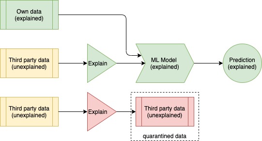

Image by author
Broken data dependencies
Somewhat self-evidently, the success of the application of an ML model depend on the performance of the data pipe and the business application. It is unlikely (and certainly undesirable) that the business application will directly affect the model, so focus on understanding data dependencies.
Broken data dependencies differ from data drift in that rather than the distribution changing, the feature itself disappears. This will be due to the feature not being generated (captured) at some point in the data pipeline. Fixing the data pipeline is the responsibility of Data Ops.
Unexpected feedback loops
Feedback can be very important in the development of ML models. However, in use unexpected feedback can cause problems. We’ve touched on an example before in the use of computed risk metrics. If we only train our model where risk is lowest, then we bias our model against certain features. This is an example of direct feedback, which when detected, can be “debugged” out.
Indirect feedback results from the use of models in the real world. The real world is a messy place, and seemingly uncorrelated (and so unmeasured) data features turn out to be very much correlated. Our flippant example earlier about toilet rolls in a pandemic caused concept drift of the pricing model.
The impact of unexpected feedback loops will generally be to degrade performance, so the identification is similar to that of drift; measure quality metrics regularly and alert when quality decays.
ML Ops toolset
Whilst model validation is the new element to master in ML Ops, there are also more conventional software engineering elements. Like all other software, ML models need to be managed in CI (continuous integration) and CD (continuous deployment) pipelines. However current CI/CD pipelines do not work well with ML projects as the steps are different. ML Ops defines model train-test for CI, validate-deploy for CD and retrain-validate-deploy for CT (continuous training) pipelines. The following table describes some key considerations for CI/CD/CT pipelines.
Humans in the loop
In the previous sections, we’ve looked at the capabilities that are needed in order to deploy an ML model. These capabilities are instantiated in sequence, in an automated pipeline, to create a deployment process flow.
Along with the automated steps, we also need some human-centric steps in our process flow:
Revert to a back-up system, normally non-ML-based but increasingly may well be a simpler ML model.
The setting of “guard rails” (action limits) is similar to the technique discussed earlier of only operating models within CVaR limits. It is up to the user to ensure that setting guard rails does not introduce unacceptable bias.
In an emergency hit the kill switch! Everything will stop and the monitoring board will light up like a Christmas tree. Such big red panic buttons are normally implemented at the infrastructure layer.
It should be noted that most global AI regulatory regimes are settling on the need to implement human-centric steps.
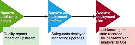
Image by author
xOps Integration
Let’s return to our definition of ML Ops: the capability to deploy and observe the right model + right data + right application, at the right time. To do all three deployments requires integration in the component operational disciplines. ML Ops is a very new discipline and we recognise that companies are at different levels of maturity in this integration.
Level 1: separate xOps
At this first level of maturity, ML models are deployed separately from business applications and data pipelines.
Data science work (data sampling, cleansing and feature engineering) and model development (selection, training, optimisation) results in algorithm and model objects to be deployed.
The business application that uses the model is developed independently. (Whether the business app is developed using Continuous Integration or Continuous Deployment techniques does not affect the development of the model.)

Image by author
The model is validated against the last known good (manually shared) version of business application using validation test data prior to deploying onto the target environment.
Additional monitoring is also deployed to observe the performance of the model. Learnings are incorporated when the next version of the model is developed.
Level 2: Integrated xOps
At the second level of maturity, data processing algorithms and ML models (or perhaps workflow objects) are deployed along with business applications and data pipelines.
As before, data science work, conducted independently of application development, results in algorithms and models to be deployed. Alternatively, the full workflow object can be deployed.
The DS objects are managed in the same repository as the application (and data archetype) objects, enabling them to be utilised together. The most recently promoted object version can be used, not just last known good version.
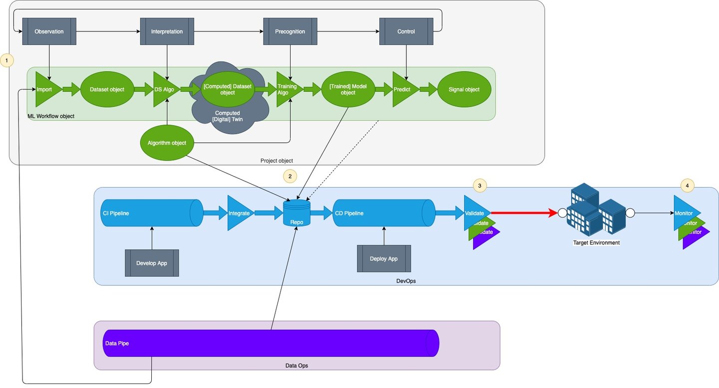
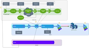
Image by author
This means the same Continuous Deployment pipeline can be used to deploy app + model + data. CD also means that validation is fully automated.
As before, additional monitoring is also deployed to observe the performance of the model. Learnings are incorporated when the next version of the model is developed.
Level 3: CI/CD/CT
At the third level of maturity, application, model and data are developed together in a continuous integration pipeline, continuously deployed, and models are maintained in a continuous training pipeline.
DS work takes place in the same Continuous Integration pipeline as application development work; the business application and the ML application are developed together.
As before, the DS objects are managed in the same repository as the application (and data archetype) objects, enabling them to be utilised together. The most recently promoted object version can be used, not just last known good version.

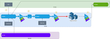
Image by author
This means the same Continuous Deployment pipeline can be used to deploy app + model + data. CD also means that validation is fully automated.
As before, additional monitoring is also deployed to observe the performance of the model. The model deals with unacceptable deviations through Continuous Training.
Conclusion: Engineering explainability is key for enterprise ML models and their deployment
This paper presents not just the need for explainability in enterprise-scale AI models, but engineering methods for explaining them. There are many strands, and all require investigation and development to fit them into the business user’s workflow. This will require equal effort into developing the models, engineering explainability and deploying into an enterprise environment with:
A suite of validation metrics, including: risk computation, chain of explainability, new safety metrics.
New approaches for continuous monitoring to assess model degradation, for cross-domain model transfer validation, for assessing infrastructure performance, and for assuring model robustness.
A toolset for source control, storage and packaging and integration into xOps through API and alarms.
An xOps maturity model that presents a grown path for enterprises.