Engineering Explainability into Enterprise AI

Explaining machine learning models: Simple rules, complex systems

The most simple neural network (NN) is very simple indeed; there are only a few parameters that describe it completely, and these parameters can be checked to assure that it has been constructed correctly. But the most simple NN doesn’t do much and isn’t very interesting. It’s when neurons are connected together, with cross-connections, feedback/feed-forward and maybe even memory cells, very interesting neural networks emerge.

These NN can learn for themselves how to interpret information and form decisions, with training. But the fact that they must be trained, not computed, means they produce a complex rule framework which cannot be analysed in its components (lacks intrinsic explainability). This black box framework is only empirically accessible, through test and measure (post- hoc explainability).

Enterprises have some key questions they want to see addressed through model explanations:

• How sensitive are the decisions to changes in inputs?

• Which inputs is the model most sensitive to?

• How transferable is the explanation of the model?

• What are the edge cases that the model may be expected to fail?

• What can be done to mitigate the impact of such failures?

These NN can learn for themselves how to interpret information and form decisions, with training. But the fact that they must be trained, not computed, means they produce a complex rule framework which cannot be analysed in its components (lacks intrinsic explainability). This black box framework is only empirically accessible, through test and measure (post- hoc explainability).

We also need to examine how the ML model interprets its data separately from explaining how it makes its decisions. Interpretability (metrics for how “easy” it is to derive predictions from data) and explainability (methods for how to relate predictions to data) are closely linked but different. Interpretability is a property of a dataset and should be calculable it from the dataset objects. Explainability is a property of a model and should be measurable it from the model + dataset objects

Overfit and learned bias

Overfit is a key contributor to learned bias. If a model is overfitting training data, and the data itself is biased with respect to the real world, then the model will be biased also. For example, if a model is able to very accurately predict a single outlier that appears in the training dataset, it will always try to predict the outlier, and the outlier is “normalised”. Put another way, if a model always predicts black swan events, it will be biased.

Overfit is best visualised in plots but commonly evaluated by measuring shrinkage, the deviation of predicted results from actual measurements. We’re investigating which shrinkage metric has the best computational efficiency, especially for arbitrarily large datasets, and how best to surface them to the user.

Image by Chabacano, CC BY-SA 4.0

Avoiding overfitting when training the model

The best way to avoid overfitting is to use training algorithms that are robust against overfitting, and to simply use more data. There are four commonly implemented engineering solutions to overfitting:

Ensemble models create multiple instances of the same ML model from different starting points. This maybe different start points within the dataset, different datasets (see next paragraph), different (random) sample of features from the full input feature set or perhaps even different loss/ activation functions. Because different approaches are taken for each model, each prediction will be different, so the output of each of the model is aggregated (perhaps a simple average) to give the final prediction. In this way, the prediction will be more robust (less overfitted), generally at the expense of accuracy.

Stratified splitting of train-test data enables us to use all of the available test-train data for training our model. We end up with an ensemble of ML models which we aggregate to give us a more robust prediction.

Regularisation (see graph above) is a technique to deliberately reduce complexity of the model to increase robustness, whilst remaining above the acceptable accuracy threshold. For example, we can reduce the contribution (weights) of features, step by step, until we reach the threshold, and see if any go to zero and so can be eliminated.

Models are developed to solve a problem, so naturally, there is a tendency to train the model with data that yields a positive prediction for the model. To balance, we should also train the model using counterfactual data, perhaps even noise, especially at the prediction threshold.

Helpfully, all of these four techniques can apply to all ML models, as they deal with how we subsample the training dataset rather than the model itself.

Training away underfit too

But what about underfit? Underfitting is often the case when sufficient volumes of training data are not available, and we can identify underfit when we see poor accuracy values in test data. We are investigating a way to tackle this by augmenting small training datasets with simulated data. For example, training a computer vision model using synthesised images overlaid on a background.

However, underfit is less prevalent than overfit. Humans are very sensitive to loss-aversion, so models will naturally be built to be more accurate than less, and therefore are more susceptible to overfit than underfit.

Approximating out bias with a DNN

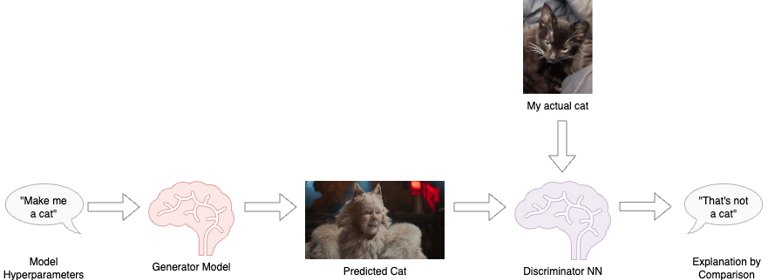
One of the approaches to quantifying bias that I’ve investigating in the past is the use of Discriminator Neural Networks (DNN) for the explanation of ML models.

The DNN is trained on similar training data to a Generator Model (GNN) but is simpler. Its job is to be able to tell the difference between generated data and actual data, so only needs to be sophisticated enough to do that job, and no more. The measured differences along selected features are the calculation of how the predictions are different from actual data, so bias can be computed and described. By varying GNN hyperparameters, the GNN can be optimised for the lowest bias.

We can take the use of DNN a step further. If the GNN proves too complex (computationally too expensive) to understand internally, then understanding the data topology of the DNN will give valuable insight, even if of a simpler proxy model. Topological Data Analysis is still pretty new, but I think it’ll be an important avenue of investigation.

Explaining datasets and features: Sampled data, biased data

Explaining the behaviour of the model is one part of ML explainability. The second, and perhaps more important part, is the explainability of the datasets.

At the scale of enterprise data problems, of ML models applied to arbitrarily large datasets, training models on the full dataset is undesirable due to the computational cost, so models are trained from samples. But whenever a sample is used, unless it is truly representative, it will be biased. So the key question becomes: how can we use the available, presumptively biased dataset to generalise predictions to new unseen datasets?

An engineering approach answers this question in two parts: first quantify the bias so that users can make an informed judgement as to how to use the data (acceptable bias); then predict the effect of bias so that users can make informed judgements as to how to use the predictions.

One can tell whether a dataset is biased by comparison; if two datasets, sampled from the same source data, have different distribution metrics then we can see that one is biased from the other. The flip side is that it is impossible to identify bias by computing the raw numbers of a single dataset without making a comparison.

Calculating comparative marginal distribution of features and comparative conditional probability distribution of two features quantifies domain divergence.

Impact of dataset bias on model predictions

Once we expect datasets to be biased due to sampling effects, understanding the impact of bias becomes the next step. The enterprise ML model should give guidance to its users as to whether the differences are acceptable, whether it’s safe to use the training data on unseen live data.

The natural next question is how the features are used in the trained model. The Partial Dependence Plot (PDP) shows how varying an “input” feature impacts the model response. It computes to a single value (commonly the average) all the samples corresponding to the x-axis value being plotted. A PDP can therefore help explain how each feature of interest (as per prior tagging, as described earlier) impacts the model’s prediction.

Comparing PDP plots of features answers explainability questions about single journeys (e.g. predictions about one person) through the model:

• Which feature influences the model the most?

• Is the amount of influence consistent over the distribution of feature values?

• Do features have undue influence?

• At what threshold value (of the feature) does the model prediction change? (Informative for categorical ML models.)

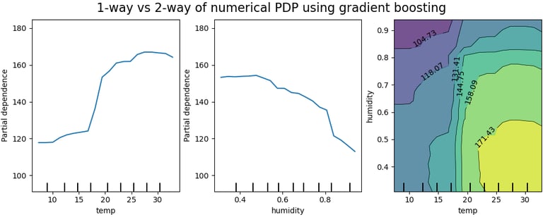
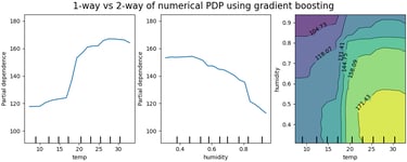
Image © 2007 - 2023, scikit-learn developers (BSD License).

Individual Conditional Expectation (ICE) plots take this a step further. An ICE plots along the y-axis the model prediction for every sample of the dataset corresponding to the x-axis value being plotted. In this way, the distribution of contribution of the feature can be visualised, not just the average. Comparing ICE plots answers the further explainability questions across all journeys (e.g. full population) through the model:

• Which features contribute high variance (equating to high uncertainty) in the prediction?

• Which features have significant outliers (which merit special treatment) in the prediction?

• Are the outcomes equitable for the full population being served?

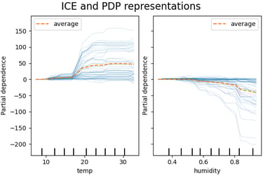
Image © 2007 - 2023, scikit-learn developers (BSD License).

All of these questions together answer whether bias makes a difference to the computed prediction, by explaining how the feature contributes to the prediction. But both these types of plots are computationally expensive and don’t work well on sparse datasets (as is often the case with fused datasets).

In a real-world solution, it’s no good to deliver bias measurements separately and later than the decisions themselves. This is where an ML engineering approach should implement approximation techniques that yield good results but more efficiently. By reducing the computation load, explainability is presented in near-real-time, so as to fit in with the user’s workflow.

Fitting explainability into an ML Ops workflow

In 2008, Google introduced its Flu Trends model that predicted the percentage US population with influenza, in time and geography. For a number of years, it outperformed the US CDC predictions, as it fused a wider range of datasets notable search terms. Except in 2012, when the model fell very short, demonstrating that even the most well-funded ML model can suffer from model drift.

“You need to be constantly adapting these models ... You need to recalibrate them every year.”

Explainability is not a one-time action, assessed by audit at the time of training the ML model. Explainability should be engineered into the full ML Ops workflow:

• Automatically set aside a third split of data dedicated to validating models before deployment;

• Computing explainability metrics and reports automatically as part of model deployment;

• API to the computing explainability metrics so that they can be triggered programmatically in life.

Explainability and privacy

At this stage it’s appropriate to inject some caution; we can’t trade explainability for privacy. For example, whilst we must be able to say how a particular feature influences a prediction, we mustn’t be able to say how a particular data point (person) influences the prediction. To protect privacy, we must implement differential privacy:

Imagine you have two otherwise identical databases, one with your information in it, and one without it. Differential Privacy ensures that the probability that a statistical query will produce a given result is (nearly) the same whether it’s conducted on the first or second database.

This is a rigorous mathematical treatment of privacy and helps us to develop engineering approaches. One such approach is to inject noise into the decision. My making the decision less precise, it is less likely to be able to trace backwards to the input. Engineering questions to investigate:

• How much noise should we add?

• Does this noise addition vary with processing of dataset (e.g. relationship with features used)?

• How do we make this calculation without having information about the dataset (and so introduce bias)?

• Which metric best calculates the trade-off between noise and accuracy, i.e. between explainability and privacy?

Conclusion: How to make explainability a key characteristic of all enterprise ML models

This paper presents not just the need for explainability in enterprise-scale AI models, but engineering methods for explaining them. There are many strands, and all require investigation and development to fit them into the business user’s workflow. This will require equal effort into engineering explainability as into developing the model themselves.